This was originally written on Nov 3, 2013, for the probability theory course I was serving as TA.
Converted from .tex using latex2wp.
Usually, we say a random variable  follows a Normal(0,1) distribution, if its cumulative distribution can be expressed as:

Now we formalize this in a more measure-theoretic way, in correspondence to what we learned in the course, particularly, why the part  is called the density of : How is the term “probability density function” that we use a lot in statistics related to the concept “density” (density of a measure with respect to another measure) that we learned in class?
First of all, we need to adopt a definition of Normal(0,1) random variable. Say is a random variable (i.e. measurable function) from  to
to  . Denote
  some probability measure on and
  the Lebesgue measure on . We say is a Normal(0,1) random variable, if we have (this is the definition we adopt, i.e. a starting point for the following arguments)
![\displaystyle P\{\omega:X(\omega)\leq t\}=\int_{(-\infty,t]}\frac{1}{\sqrt{2\pi}}e^{-\frac{x^{2}}{2}}d\mu(x). \ \ \ \ \ (1)](https://s0.wp.com/latex.php?latex=%5Cdisplaystyle+P%5C%7B%5Comega%3AX%28%5Comega%29%5Cleq+t%5C%7D%3D%5Cint_%7B%28-%5Cinfty%2Ct%5D%7D%5Cfrac%7B1%7D%7B%5Csqrt%7B2%5Cpi%7D%7De%5E%7B-%5Cfrac%7Bx%5E%7B2%7D%7D%7B2%7D%7Dd%5Cmu%28x%29.+%5C+%5C+%5C+%5C+%5C+%281%29&bg=f7f3ee&fg=000000&s=0&c=20201002)
Now, how to convert this into a statement that is the density of some measure with respect to some other measure? Note that when saying some function  is the density of some measure
  with respect to some other measure , and need to be defined on the same measurable space, so at this point we cannot say is the density of with respect to .
But now the distribution comes to rescue. Recall that at some ealier time point of the class, we’ve learned the concept “distribution” of a random variable, which is a measure  on the target space (here ) defined as following: for any
  ,
,

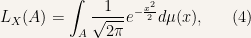
So by (1) we have
![\displaystyle L_{X}((-\infty,t])=\int_{(-\infty,t]}\frac{1}{\sqrt{2\pi}}e^{-\frac{x^{2}}{2}}d\mu(x), \ \ \ \ \ (3)](https://s0.wp.com/latex.php?latex=%5Cdisplaystyle+L_%7BX%7D%28%28-%5Cinfty%2Ct%5D%29%3D%5Cint_%7B%28-%5Cinfty%2Ct%5D%7D%5Cfrac%7B1%7D%7B%5Csqrt%7B2%5Cpi%7D%7De%5E%7B-%5Cfrac%7Bx%5E%7B2%7D%7D%7B2%7D%7Dd%5Cmu%28x%29%2C+%5C+%5C+%5C+%5C+%5C+%283%29&bg=f7f3ee&fg=000000&s=0&c=20201002)
or (by some careful treatment of the fact that  is the sigma-field generated by all half-infinity intervals and the properties of measure)
for any .
That is to say, is the density of (distribution of , which is a probability measure) with respect to (the Lebesgue measure on the real line).
